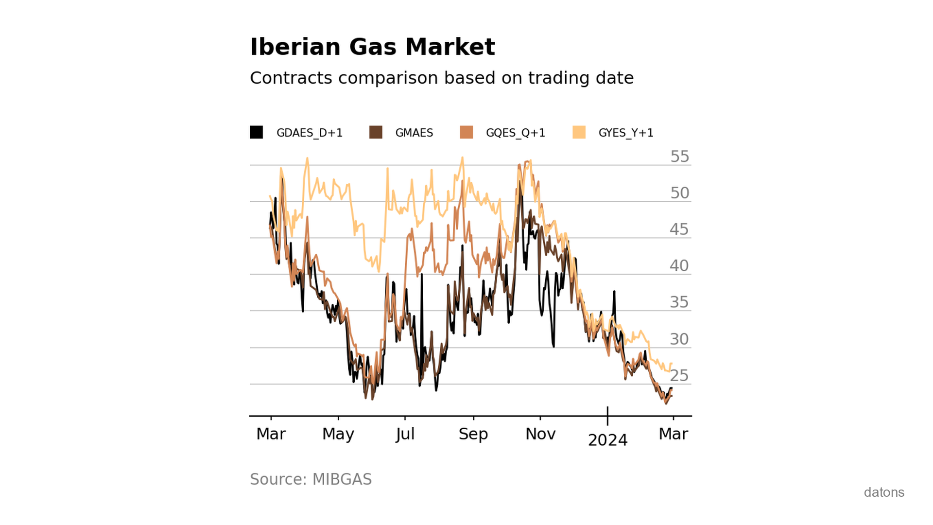
If I have a factory that consumes natural gas, it’s not the same to buy it for consumption the next day as for the next year. Prices vary depending on the delivery date, and it’s important to have an overview of how they behave to make purchasing decisions.
In Figure 1, we see that, in general, future prices are higher than current prices. This is known as contango.
As they say in Argentina: it takes two to tango.
All very clear, but… how do we process the raw data provided by MIBGAS for a contract comparison visualization?
Data
Each row represents a trading date for a specific contract depending on when the gas will be delivered.
- GDAES_D+1: Next day
- GMAES: Next month
- GQES_Q+1: Next quarter
- GYES_Y+1: Next year
In this tutorial, we work with 2024 data in CSV format, obtained from MIBGAS.
import pandas as pd
df = pd.read_csv('data/MIBGAS_Data_2024.csv', sep=';', skiprows=1)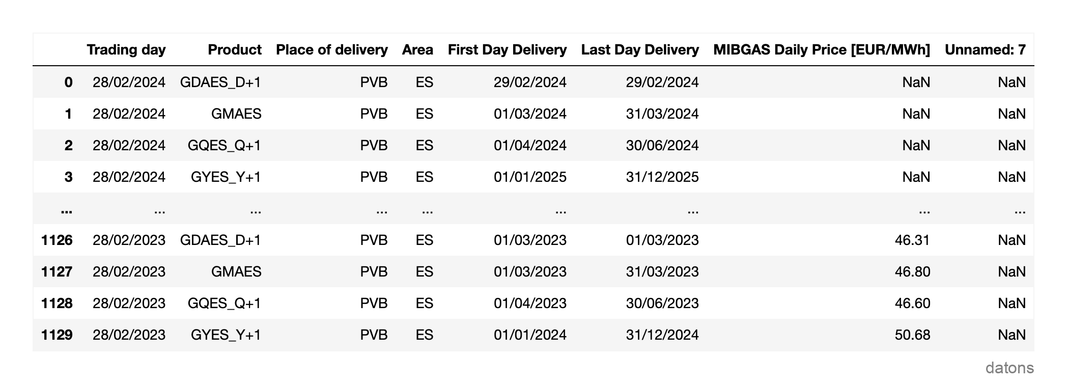
Questions
- Why filter and rename the columns of the
DataFrame? - How do we restructure the contract categories into columns of the
DataFrame? - What function is used to convert text to dates?
- How to visualize data directly from the
DataFramewith a function? - What smart technique is applied to fill missing data in time series?
- Why is it important for the time series to be sorted by date?
Methodology
Select and rename columns
We will compare the different gas prices by contract type and trading date.
df = df.filter(regex='Trading|Product|MIBGAS')
df.columns = ['date_trading', 'contract', 'price']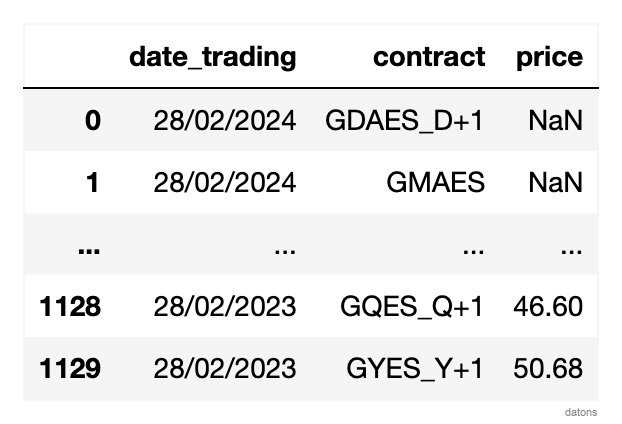
Restructure contracts into columns
To simplify working with the DataFrame, we will restructure it so that each column represents a contract and each row a trading day.
df = df.pivot(index='date_trading', columns='contract', values='price')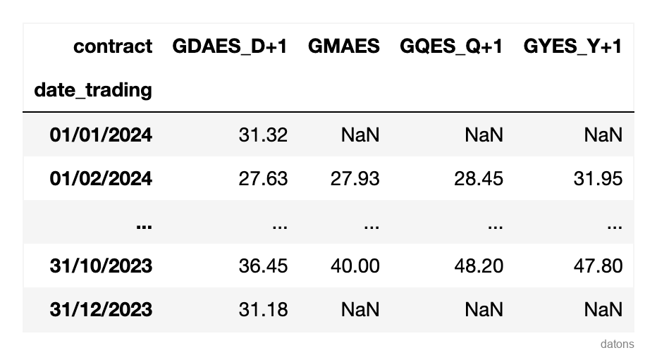
Format date column
By default, dates are in string format. We will convert it to datetime so that visualization and analysis functions take into account the temporal nature of the data.
df.index = pd.to_datetime(df.index, dayfirst=True)Sort rows by date
It is very important that the data is sorted by date so that visualization is done in the correct order.
df.sort_index(inplace=True)Comparative column visualization
Since the pandas DataFrame is connected to the matplotlib library, we can visualize the data directly using the plot function.
df.plot();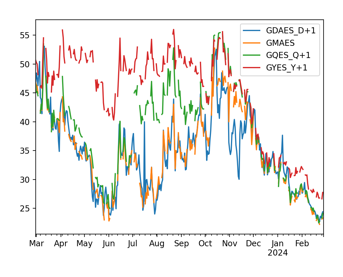
We observe many irregular jumps due to missing data on some days, probably due to holidays or weekends.
Linear interpolation
We will use linear interpolation to fill these gaps, making the visualization clearer.
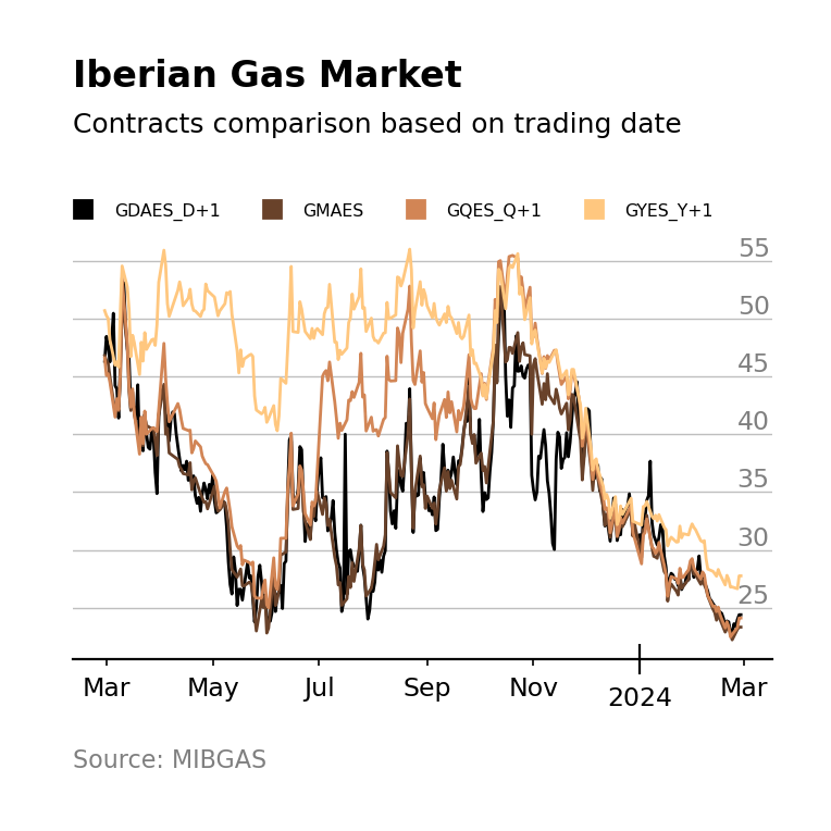
df.interpolate(method='linear', inplace=True)Now we can compare the different gas contracts over time.
If we observe that lighter colors indicate a more distant horizon and are mostly positioned at the top of the graph, we can conclude that, in the long term, gas prices are higher.
Conclusions
Thanks to this tutorial, you now know how to:
- Filter & Rename Columns: Simplify the
DataFrameto work only with the variables you’re interested in and rename them for easier handling. - Restructure DataFrames: The
pivotfunction allows you to restructure categories from one column into independent columns, simplifying data visualization and analysis. - Transform Text to Dates: Using
pd.to_datetimeto convert strings todatetimeobjects is essential for efficiently manipulating time series. - Data Visualization: The integration of
PandaswithMatplotlibenables direct and effective visualizations from theDataFrame. - Linear Interpolation: Linear interpolation is a key technique for dealing with missing data, allowing for a continuous representation of time series.
- Sort Time Series: It’s crucial to sort data by date to ensure temporal coherence in analysis and visualization.
Keep reading
Related articles you might enjoy
Unstack data frame after grouping to create heat matrix
Python tutorial to unstack the row categories into columns (long to wide table) to later create a heat matrix.
Read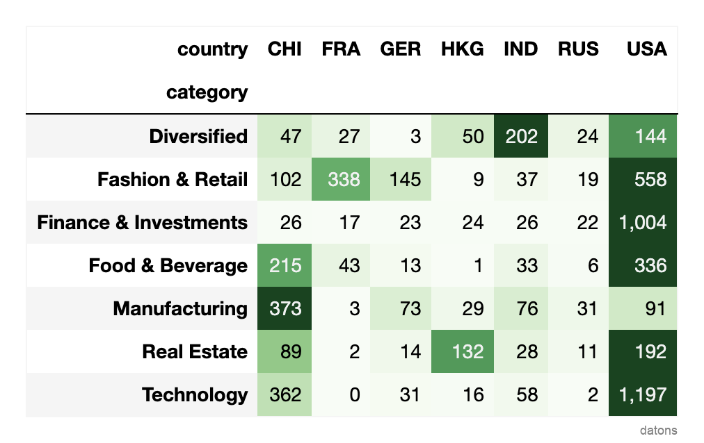
Style pivot table to create heat matrix
Learn how to highlight the most valuable cells in a Pandas pivot table that summarizes information on billionaires by country and industry.
Read
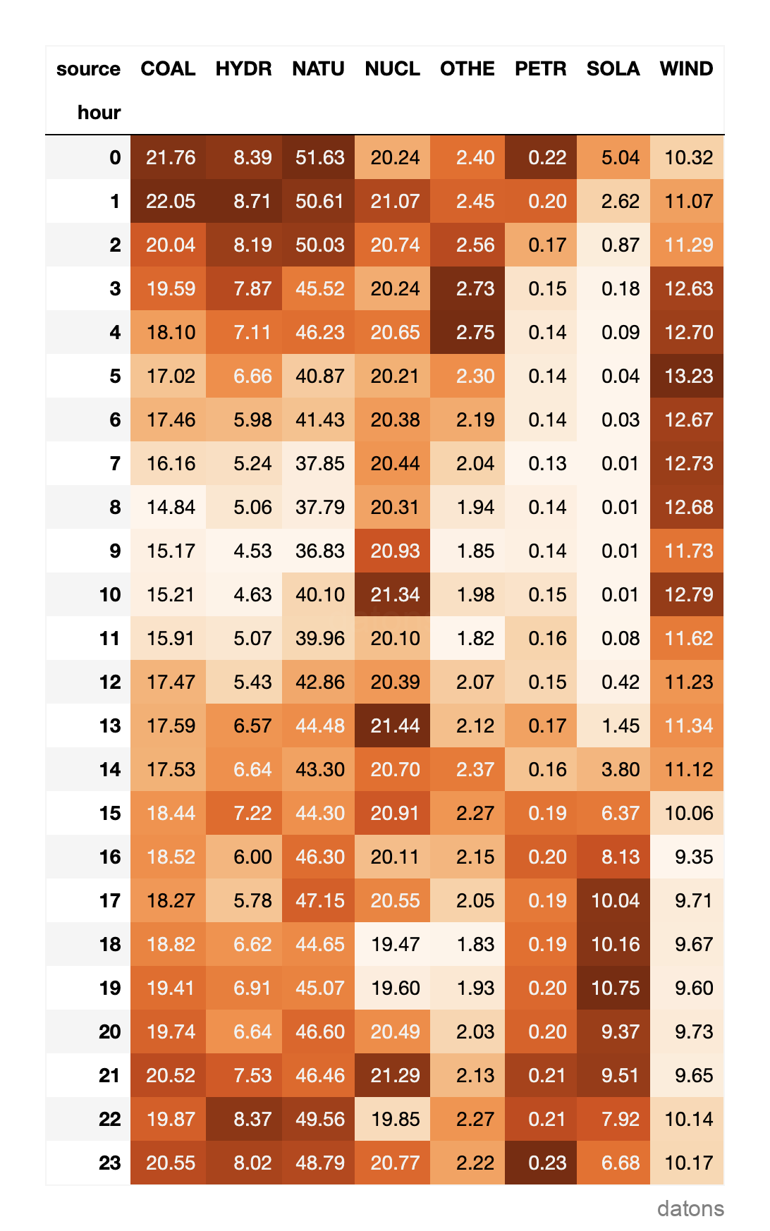
Working with temporal properties using pandas Datetime Index
Leverage the properties of DatetimeIndex in Pandas for more efficient time series analysis, from formatting the column to creating reports with pivot tables.
Read